§ I. the number
Begin with the observation as given, stripped of interpretation. A fixed reference task, the same kind of result held to the same standard of rigor, required one year at time \(t=0\) and requires one week at \(t=5\), with \(t\) measured in years. Assume, as a first hypothesis, that the compression was steady: that the time-to-completion \(T(t)\) decayed exponentially,
The boundary condition \(T(5) = \tfrac{1}{52}\) yr fixes the single parameter,
so that \(T(t) = 52^{-t/5}\) and the speedup factor is its reciprocal, \(S(t) = 52^{\,t/5} = e^{0.790\,t}\). Two invariants are worth carrying in the pocket. The doubling time of productivity is \(\tau_2 = \ln 2/\lambda \approx 0.877\) yr, call it ten and a half months, and the annual compounding factor is \(52^{1/5} \approx 2.20\). A person on this curve is not improving; they are doubling, on a cadence slightly faster than the seasons repeat.
And yet, for all its drama, this curve is tame. Define the instantaneous growth rate \(g(t) = \frac{\dd}{\dd t}\ln S\). Here \(g \equiv \lambda\): a constant. The future, on this hypothesis, is merely a faster version of the present, at every horizon, forever. Hold that flatness in mind. It is the quantity everything below will bend.
§ II. many hands
Now suppose there are \(N\) such people. If each produces output at rate \(r(t) = r_0 e^{\lambda t}\) and they work independently, the aggregate is
with the familiar corollary that each doubling period produces as much as all prior history combined. But note what \(N\) does not do: it shifts the curve without changing its shape. The exponent is untouched. Population is a prefactor; it cannot, by itself, make history curve.
Two refinements can. First, heterogeneity. If the personal rate \(\lambda\) varies across the population with density \(f(\lambda)\), then
the moment generating function of the rate distribution, and the effective exponent
is increasing in \(t\). The fastest adopters weigh ever more heavily in the average, so the aggregate is superexponential even though every individual, examined alone, is merely exponential. If \(f\) has tails as fat as an exponential distribution’s, \(M_\lambda(t)\) diverges at finite \(t\): a singularity manufactured from variance alone, with no feedback anywhere in the mechanism. Second, coupling. If the workers amplify one another through shared instruments and results compounding across a network, write \(P = N^{1+\gamma} r_0 e^{\lambda t}\) with \(\gamma > 0\) for superlinear returns to scale; let adoption itself spread, \(N(t) = N_0 e^{\mu t}\), and the transient exponent becomes \(\lambda + (1+\gamma)\mu\), visibly steeper than any participant’s. The moral is compact: \(N\) multiplies, but variance and coupling bend. An observer inside such a population sees ordinary exponential improvement in the mirror and something faster than exponential out the window, and both observations are correct.
§ III. the horizon
What, then, would the genuine article look like, the curve the word singularity was coined for? The answer is one structural alteration. In everything above, the exponent was exogenous: the tools improve the worker, but the worker’s output does not feed back into the rate at which the tools improve. Endogenize it. Let output include improvements to the improver, \(\lambda = \lambda(P)\), and take the minimal version \(\lambda(P) = \kappa P^{\varepsilon}\):
Hyperbolic, not exponential: finite-time blowup at \(t^{*}\). And observe the knife-edge. At \(\varepsilon = 0\) exactly, the equation returns the tame curve of § I, valid for all time; for any \(\varepsilon > 0\), however small, the solution has a last date. The entire question compresses into a single bit, whether the exponent’s exponent is zero, and exponential growth, which feels so violent from inside, is revealed as the boundary case: the fastest a system can grow while still possessing a future at every date.
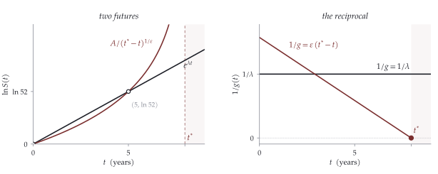
The two regimes are distinguishable in data, and by an instrument of almost embarrassing simplicity. Plot the reciprocal of the growth rate:
a straight line descending to zero, whose \(x\)-intercept is the date of the singularity. Figure I renders both faces of the dilemma: two curves that agree on every observation made so far, and disagree about the existence of an eighth year.
This is not a hypothetical procedure. In 1960, von Foerster and colleagues ran precisely this regression on two millennia of world population and found \(N(t) \approx C/(t^{*}-t)^{0.99}\), an almost perfect hyperbola, with intercept \(t^{*} =\) November 13, 2026. As these notes are written, that date lies some sixteen weeks ahead. Humanity was excused from the appointment by the demographic transition: growth went sub-hyperbolic after 1970, and the best-fitting curve of 1960 quietly ceased to describe the world that contained it. The lesson survives the reprieve. A superbly fitting hyperbola tells you about the regime you are in, not the regime you will stay in.
There is a standard mechanism for such reprieves, and it is worth stating because it decides where acceleration lands first. Let output require several essential inputs combined with elasticity of substitution \(\sigma < 1\): complements, not substitutes. Then growth is asymptotically pinned to the slowest essential input: Baumol’s drag. If even one indispensable task resists automation (anywhere verification is expensive, anywhere ground truth takes a laboratory or a decade), the hyperbola flattens into a sigmoid. On this view the fields transforming fastest today are not evidence that the horizon is general; they are the fields in which every essential input happens to verify cheaply, the \(\sigma\)-sorted front of the wave. The aggregate question, blowup or Baumol, turns on whether the expensive-to-verify residue is truly essential, or merely traditional.
§ IV. the flywheel
Return, finally, to the single researcher of § I, and complicate the story in the one way honesty requires. The five-year compression was not produced by practice alone. The instrument improved, and it improved in part because it was fed the researcher’s own output. Decompose the log-speedup into a personal term and an instrumental term, \(S(t) = e^{u(t) + v(t)}\), with dynamics
The second equation is the revision that matters: the instrument’s gains are driven by data, and the data rate is the current speed. Substituting \(u = at\) and setting \(w = e^{-v}\) linearizes the system, \(\dot w = -c\,e^{at}\), giving the closed form
The structure of this solution deserves a slow look. As \(c \to 0\) it collapses to the innocent exponential of § I, valid forever. For any \(c > 0\), the denominator reaches zero at
and the solution is finite-time singular, even though the personal learning rate was held to a constant. The hyperbolic regime is not contributed by either component; it emerges from the coupling. A person can be entirely ordinary, improving at a fixed exponential clip, and still be a working part of a system with a last date.
Now the uncomfortable epistemology. The observed trajectory imposes one constraint, \(S(5) = 52\), that is,
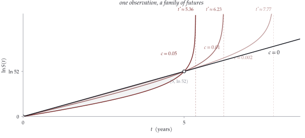
one equation in two parameters. The decomposition into my improvement and the instrument’s improvement from my data is unidentifiable from the time series alone; every division of credit is consistent with the curve. Separation requires a counterfactual arm: one’s speed against a frozen instrument (\(c = 0\)) identifies \(a\), and the residual is the flywheel. Absent that, a single testable fingerprint remains: the coupled model predicts that \(\ln S(t)\) is convex, since feedback back-loads the gains, while pure personal improvement predicts a straight line. The question one’s own history can answer is whether the passage from year to week was uniform in log-time, or whether the final year contributed out of all proportion. Convexity is the flywheel confessing. Figure II makes the indeterminacy visible: a family of histories, every member calibrated to the same five years, each convex curve dipping below the chord exactly as convexity requires, and each carrying a different last date.
One aggregation, and the account closes. With \(N\) contributors feeding the same shared instrument, the coupling scales as \(c \mapsto Nc\), so
The horizon approaches linearly in the number of hands. This, formalized, is the sense in which the present instrument differs from every prior one: the lathe made its operator faster, but one machinist’s afternoon never shortened another’s; here the tool is shared, so each person’s use compounds into everyone’s rate, and the remaining distance to \(t^{*}\) is divided among all who touch it.
Coda. The strange property of the distinction drawn here is that it is invisible at any single moment. Stand at time \(t\) inside either regime and the view is identical: things are fast, and getting faster. The difference between \(e^{\lambda t}\) and \(A/(t^{*}-t)^{1/\varepsilon}\) lives entirely in the future, which is to say, in a quantity that must be inferred, never witnessed. But the inference is available, and it asks almost nothing. Keep a private record of the growth rate of your own capability. Take its reciprocal. Hold a ruler to it. If the line is flat, you are living in an era, however astonishing. If it slopes, note where it crosses zero, without alarm and without disbelief. Fifty-two was a conversion factor between a year and a week. The next number of interest is an intercept.