1.A small move with a long reach

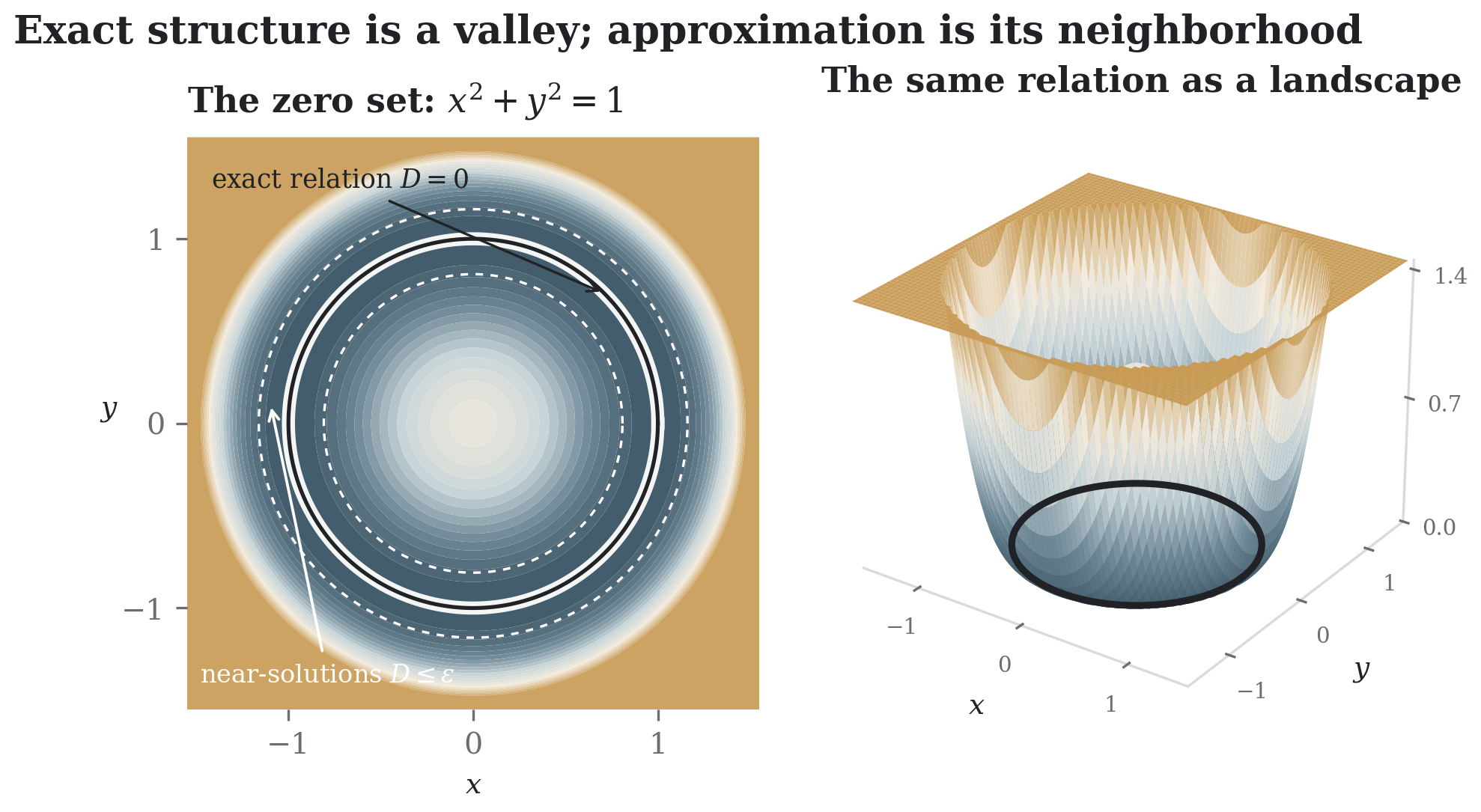
Begin with a circle. The equation \(x^2+y^2=1\) draws a perfect boundary: a point lies on it or does not. Now square the failure, \[D(x,y)=(x^2+y^2-1)^2.\] Nothing on the circle has moved, yet everything around it has changed. Points that were merely “not on the circle” now occupy slopes and level curves. Exactness has become the floor of a landscape.

This move is so familiar that it is easy to miss its audacity. Euclid organized geometry through exact constructions, equality, congruence, and ratio [4]. Modern mathematics repeatedly asks one question more: when a configuration is not exact, how does it fail? Equality becomes error, an equation becomes a residual, and a hard constraint becomes a loss. The sharp object remains; around it appears a geometry of near misses.

Ordinary distance is the elementary instance. It turns \(x=y\) or \(x\ne y\) into a scale \(d(x,y)\), from which neighborhoods, limits, and continuity follow. But the farther the idea travels, the less often two points are enough. Addition is the ternary relation \(a+b=c\); incidence joins a point and a line; a field equation judges a function. The pairwise metric therefore gives way to \[D_R:X_1\times\cdots\times X_n\to[0,\infty),\qquad R(x_1,\ldots,x_n)\Longleftrightarrow D_R(x_1,\ldots,x_n)=0.\] At its cheapest, \(D_R\) is \(0\) when \(R\) holds and \(1\) when it fails. That is only a change of costume. The serious cases begin when the positive values carry knowledge: when \(0.01\) and \(100\) locate genuinely different kinds or degrees of failure.

The essay will carry one instrument into several territories. Each time we will ask \[\boxed{\text{objects}\;|\;\text{relation}\;|\;\text{discrepancy}\;|\;\text{zero set}\;|\;\text{neighborhood}.}\] The identical form matters. It lets us see which examples are nearly free, which demand a sacrifice, and which reveal a theorem. Arithmetic already comes with subtraction. Order forces us to abandon symmetry. Logic must be given a notion of graded failure. Approximate algebra confronts the hardest question of all: whether an object that nearly obeys a law is actually near one that obeys it exactly.

2.Before distance had a number

The thought that geometry might begin with relation rather than magnitude is older than the modern language needed to state it. In a 1679 letter to Huygens, Leibniz proposed an analysis situs: a geometry of position that would attend to situation before size. Huygens was not persuaded [16]. Decades later, in the Leibniz–Clarke correspondence, Leibniz described space as an order of coexistences, opposing the Newtonian picture of an absolute container in which things happen [15]. He did not anticipate discrepancy functions. His role here is more interesting than that: he made it conceivable that geometry could live in the pattern among things rather than in a substance called space.

The idea acquired machinery in stages. Descartes’ La Géométrie allowed an equation to carry the form of a curve [3]. Riemann’s 1854 habilitation lecture went deeper: the manner of measurement could itself be mathematical data, varying from place to place [20]. Then Fréchet, in 1906, isolated an abstract écart between arbitrary elements, retaining what analysis needed for convergence while forgetting what the elements were [6]. The word “point” quietly expanded. It could now mean a graph vertex, a string, a function, or a probability distribution. Geometry had escaped the room of physical space without ceasing to be geometry.

Leibniz’s Identity of Indiscernibles now returns with mathematical force. The metric axiom \[d(x,y)=0\Longrightarrow x=y\] is the principle in arithmetic form: nothing distinct is perfectly indistinguishable. A pseudometric deliberately relaxes the demand, permitting \(x\ne y\) while \(d(x,y)=0\); quotienting by zero distance restores the principle by construction. This is more than a technical distinction. Every discrepancy makes a decision about reality. If two signals differ only by a phase the model ignores, or two parameter settings produce the same observable behavior, zero discrepancy declares that difference immaterial. Measurement does not merely report a world already divided. It helps decide which divisions the theory can see.

3.Algebra enters the landscape

Geometry has now been freed from physical space, but algebra still appears to stand apart. Its basic act is not comparison but composition: take \(a\) and \(b\), and produce \(a\circ b\). The distance viewpoint becomes useful only after we stop staring at the inputs and look at the whole multiplication triple.

Here the obvious objection cannot be postponed. If \(D_\circ\) takes only the values \(0\) and \(1\), we have merely renamed truth as zero. The landscape earns its name only when its heights expose questions that the exact law concealed: how much must a product change to restore associativity? Where does a law fail most severely? Does small local defect place us near any globally exact algebra at all?

That last question became a subject in 1940, when Ulam asked whether a map that almost preserves group multiplication must lie near an exact homomorphism [24]. Hyers answered the following year in a foundational setting: between Banach spaces, a uniformly approximately additive map lies uniformly near an exactly additive one [10]: \[\|f(x+y)-f(x)-f(y)\|\leq\delta\quad\Longrightarrow\quad\|f(x)-A(x)\|\leq\varepsilon\] for an additive \(A\), with appropriate constants. In this theorem the metaphor hardens: a thickened law really does contain a nearby exact law. But the subsequent stability program also found equations for which this promise fails [18]. The landscape may slope toward an exact structure, or it may not. Drawing the landscape is easy; discovering when its low ground tells the truth is mathematics.

4.When observations refuse to meet

For equations, the apparatus is almost embarrassingly cheap. Subtraction already measures failure. Yet this easy case produced one of the decisive turns in the history of applied mathematics, because the heavens would not cooperate with exactness.

Astronomical observations made this last step unavoidable. Measurements of the same orbit did not pass through one immaculate curve; each arrived with error, and together they could be inconsistent. Legendre first published least squares in 1805. Gauss, publishing in 1809, claimed to have used the method since 1795 [14, 7]. The priority dispute is less revealing than the shared necessity. Faced with observations that refused to intersect, mathematics did not discard the problem. It made inconsistency into terrain and asked which point lay lowest.

The same move can be watched in miniature. Require a Boolean variable \(x\) to satisfy both \(x=0\) and \(x=1\), giving the second demand twice the weight. Exact satisfiability has nowhere to go: the zero set is empty. Relax \(x\in[0,1]\) and minimize \[\begin{aligned} L(x)&=x^2+2(x-1)^2=3x^2-4x+2,\\ L'(x)&=6x-4.\end{aligned}\] Thus \[x^\star=\frac23,\qquad L(x^\star)=\frac23.\] The number \(2/3\) is not a third truth value. It is a location: the point where incompatible demands balance under the chosen geometry. Change the weights and the point moves. That dependence is not an embarrassment; it records what the model has decided to care about.

5.The price of softening truth

Equation residuals arrive with a natural scale. Logic does not. A false proposition is false; classical truth offers no native answer to “by how much?” The next extension therefore costs something: a semantics of violation must be designed rather than uncovered.

Fuzzy logic, many-valued logic, and continuous relaxations all make versions of this bargain [25]. They gain comparison and motion, but only by adding structure to truth. Two softenings may agree perfectly on which assignments are exact and disagree everywhere nearby. Their optimizers can diverge. The zero set does not choose its own hills.

6.A geometry that points one way

Order presents a different resistance. Distances are expected to be symmetric, but “no greater than” has an arrow built into it. The way forward is not to erase that arrow. It is to let geometry inherit it.

The two directions answer different questions, and that asymmetry is the information. Lawvere’s 1973 construction makes the unity exact. Turn the usual order on \([0,\infty]\) around and use addition as composition. A category enriched over this base assigns a value \(d(x,y)\) to every ordered pair; its rule for composition is \[d(x,y)+d(y,z)\geq d(x,z),\] which is precisely the triangle inequality. Symmetry and separation are optional. Collapse the base to \(\{0,\infty\}\) and the same architecture becomes a preorder: \(d(x,y)=0\) means \(x\preceq y\) [13]. With suitable bases, logical conjunction and implication also arise from the monoidal closed structure. Here the essay’s sweeping resemblance is no longer only a resemblance. Metric, order, composition, and logic occupy neighboring rooms in one formal house.

7.From paths to landscapes

So far the candidate configurations have been finite: a triple, an assignment, an ordered pair. But a mathematical object can also unfold in time. Once an entire path is treated as one point in a larger space, a differential equation becomes a relation on histories.

Physics supplied this language long before the modern word “loss” became ubiquitous. Euler, Lagrange, and Hamilton learned to compare whole possible motions through extremal principles; Ritz turned the same idea into a method of approximation [5, 12, 9, 21]. The actual motion appears not as a point selected by a local rule alone, but as a privileged history among neighboring histories.

Machine learning inherits this lineage through least squares, likelihood, and regularization [22, 23]. Its especially suggestive move is that descent can alter not only a prediction but the representation in which later predictions will be compared. The landscape helps build the eyes that inspect it. And landscapes can deceive: they contain spurious minima, broad plateaus, and thin curved trenches. Such features are invisible from the zero set alone. Here the surrounding geometry is not decoration; it determines whether learning can find its way.

8.Distinguishing possible worlds

Probability changes the mood of the question. The objects are no longer single outcomes but entire accounts of what might happen. To compare two distributions is to ask how readily evidence can tell their possible worlds apart.

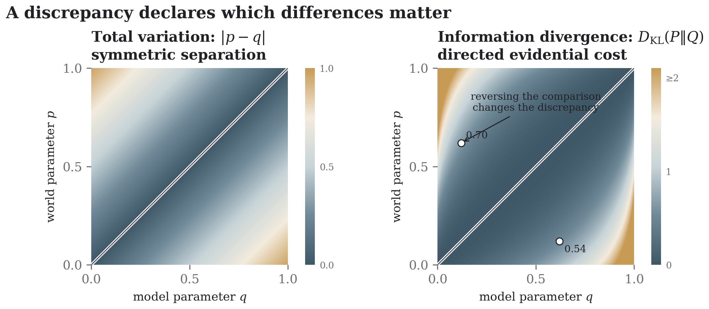
The asymmetry of KL divergence is not a flaw waiting to be repaired. Expectations weighted by \(P\) ask what happens when \(P\) is the world and \(Q\) is the approximation; reversing them asks another question. A mismatch of support may even make one direction infinite while leaving the other finite. Kullback and Leibler tied this directed quantity to information and sufficiency [11]. Rao had already shown that a smooth family of statistical models carries a local geometry through information [19]. Evidence, estimation, and coding had discovered their own notions of near and far.

9.The staircase of objects

There is now a pattern beneath the pattern. Each time mathematics learns to handle a kind of object, it can place many such objects into a new space and begin comparing them. Numbers become coordinates of vectors; functions become points in normed spaces; distributions become points in statistical manifolds. Graphs, algebras, and eventually whole metric spaces become candidates for geometry in their own right. Banach helped consolidate complete normed spaces of functions; Gromov made entire metric spaces comparable [1, 8].

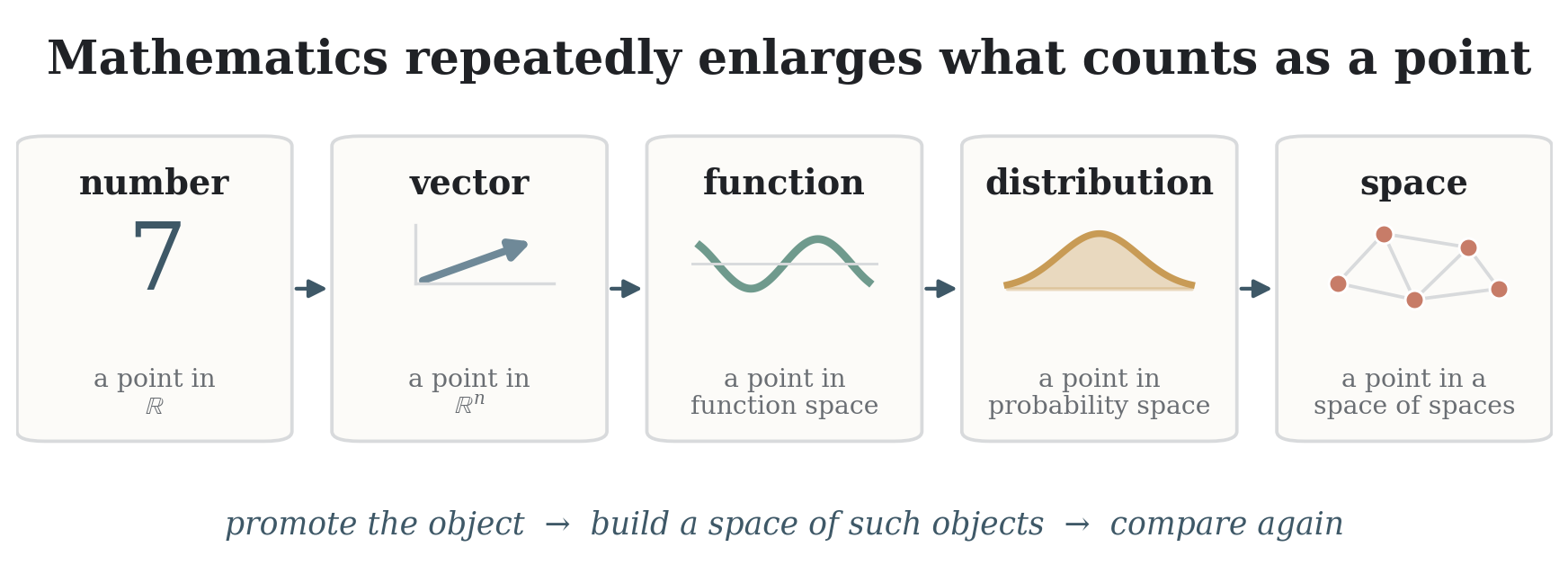
The ascent has a simple rhythm: \[\text{objects}\to\text{space of objects}\to\text{discrepancy on that space}\to\text{new structure}.\] Then the new structure itself becomes an object, and the question begins one level higher. Mathematics repeatedly enlarges what can count as a point without exhausting the question of what it means for two points to differ. This recursion is why the distance idea seems to wait for us wherever we arrive.

10.At the edge of the map

A view this broad carries its own danger. Any relation admits a \(0/1\) indicator; any finite table can be disguised as a zero set. If mere encodability were enough, the thesis would explain everything and therefore nothing. A useful discrepancy must answer for its positive values. It should justify a scale, a topology, an operational interpretation, or—best of all—a theorem showing that small defect controls something the original subject values.

Leibniz’s characteristica universalis offers an apt historical warning. A universal symbolic language may aspire to express every dispute without possessing the resources to decide any of them [17]. The same temptation shadows every universal vocabulary. Hyers’s theorem escapes it because a small defect yields a nontrivial nearby exact object; unstable equations sharpen the achievement by showing it could have been otherwise. Lawvere’s enrichment escapes it because the common form is proved, not proclaimed. The elementary relaxation escapes it because it returns \(2/3\) and shows openly which choices made that answer possible.

Nor can every important feature be pressed into one scalar. Two discrepancies may share a zero set and disagree everywhere else. A topology may have no preferred metric; algebraic composition contains information no ordinary pairwise distance recovers; logical consequence is not simply numerical closeness. The phrase “geometry of distinguishability” is strongest not as a conquest but as an invitation: what distinctions does a theory recognize, which can be graded, what does the grading preserve, and what becomes visible only after the exact boundary is allowed to have a neighborhood?

11.Where geometry begins

We can now return to a familiar sentence:

The journey adds one quiet move. A relation can often be regarded as the zero set of a meaningful discrepancy. The relation tells us which configurations are exact; the discrepancy lets the surrounding possibilities speak.

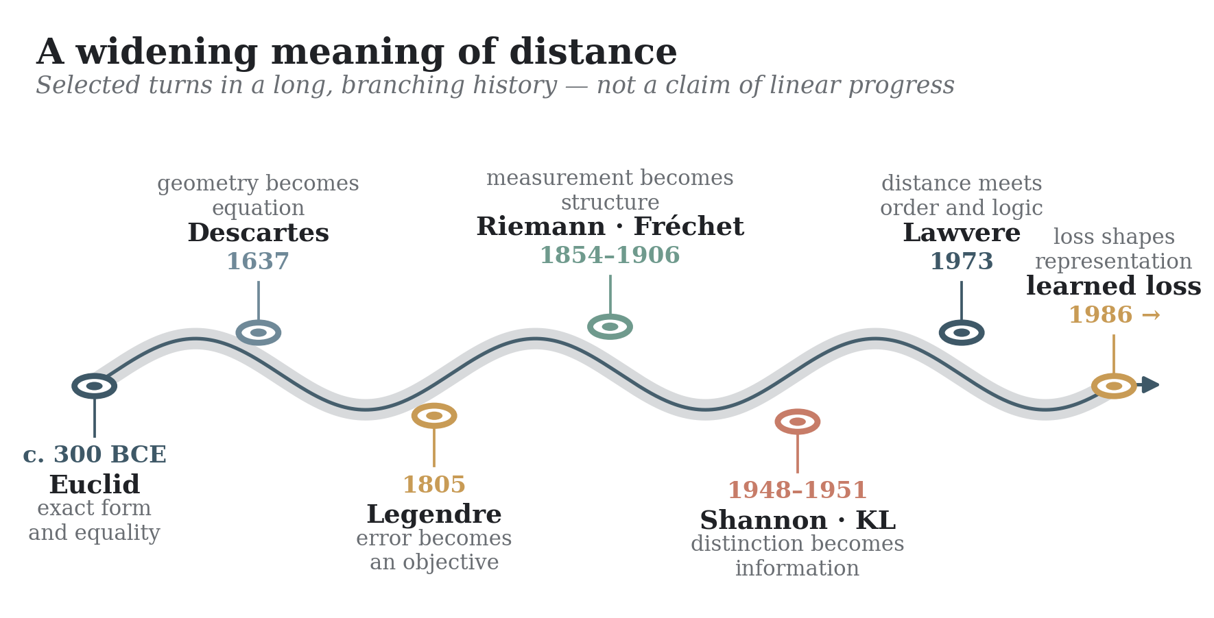
Seen this way, the history has a remarkable shape. Euclid organized exact configurations. Leibniz imagined a geometry of relation and position. Descartes allowed equations to draw. Legendre and Gauss found a disciplined answer when observations would not meet. Riemann and Fréchet made measurement itself mathematical. Birkhoff foregrounded systems of laws. Rao and Kullback–Leibler made statistical distinction geometric and informational. Ulam and Hyers asked whether almost lawful objects live near lawful ones. Lawvere showed distance, order, composition, and logic meeting inside one formal architecture. Modern learning turned discrepancy into an engine that can remake its own representation.

The simplicity is almost disorienting. Ordinary geometry measures separation. Analysis measures approach to limits. Optimization measures departure from optima. Algebra can measure deviation from laws. Logic can grade constraint violation. Statistics compares possible worlds. Physics orders histories by action and states by energy. Computation turns constraints into losses. Then functions, distributions, graphs, algebras, spaces, and histories themselves become points, and the question returns: \[\boxed{\text{How different are these two things---or these two configurations?}}\] No ordinary pairwise metric contains all of operation, order, logic, and relation. That is precisely why the enlargement matters. Relational discrepancy does not flatten those subjects into one object; it lets us recognize a shared passage from exactness to approximation, from membership to neighborhood, from a law to the shape of its possible failure.

That may be the real reason distance appears everywhere. Mathematics does not secretly live in Euclidean space. It is perpetually deciding what may count as the same, what must count as different, and which differences matter enough to measure. Each such decision opens a local geometry.

The journey from Euclid’s exact circle to a learned loss landscape is therefore not a march away from geometry. It is geometry discovering, century by century, that its deepest subject was never only space. A circle becomes an equation; an error becomes a direction; a law acquires a neighborhood; a possible world becomes distinguishable from another. Beneath the changing apparatus, the same small question keeps opening larger rooms.

References

- S. Banach, Théorie des opérations linéaires, Warsaw, 1932.
- G. Birkhoff, “On the structure of abstract algebras,” Proc. Cambridge Philos. Soc. 31 (1935), 433–454.
- R. Descartes, La Géométrie, Leiden, 1637.
- Euclid, The Thirteen Books of the Elements, trans. T. L. Heath, 2nd ed., 1926.
- L. Euler, Methodus inveniendi lineas curvas, 1744.
- M. Fréchet, “Sur quelques points du calcul fonctionnel,” Rend. Circ. Mat. Palermo 22 (1906), 1–74.
- C. F. Gauss, Theoria motus corporum coelestium, Hamburg, 1809.
- M. Gromov, Metric Structures for Riemannian and Non-Riemannian Spaces, 1999.
- W. R. Hamilton, “On a general method in dynamics,” Phil. Trans. R. Soc. 124 (1834), 247–308.
- D. H. Hyers, “On the stability of the linear functional equation,” PNAS 27 (1941), 222–224.
- S. Kullback and R. A. Leibler, “On information and sufficiency,” Ann. Math. Stat. 22 (1951), 79–86.
- J.-L. Lagrange, Méchanique analitique, Paris, 1788.
- F. W. Lawvere, “Metric spaces, generalized logic, and closed categories,” Rend. Sem. Mat. Fis. Milano 43 (1973), 135–166.
- A.-M. Legendre, Nouvelles méthodes pour la détermination des orbites des comètes, Paris, 1805.
- H. G. Alexander, ed., The Leibniz–Clarke Correspondence, 1956.
- V. De Risi, Geometry and Monadology: Leibniz’s Analysis Situs and Philosophy of Space, 2007.
- G. W. Leibniz, Logical Papers: A Selection, trans. M. Parkinson, 1966.
- Z. Moszner, “On the stability of functional equations,” Aequationes Math. 77 (2009), 33–88.
- C. R. Rao, “Information and the accuracy attainable in the estimation of statistical parameters,” Bull. Calcutta Math. Soc. 37 (1945), 81–91.
- B. Riemann, “Über die Hypothesen, welche der Geometrie zu Grunde liegen,” lecture of 1854, published 1868.
- W. Ritz, “Über eine neue Methode zur Lösung gewisser Variationsprobleme,” J. Reine Angew. Math. 135 (1909), 1–61.
- F. Rosenblatt, “The perceptron,” Psychological Review 65 (1958), 386–408.
- D. E. Rumelhart, G. E. Hinton, and R. J. Williams, “Learning representations by back-propagating errors,” Nature 323 (1986), 533–536.
- S. M. Ulam, A Collection of Mathematical Problems, 1960.
- L. A. Zadeh, “Fuzzy sets,” Information and Control 8 (1965), 338–353.