Quantum-Accelerated Stabilization for Markov-Chain Averaging

Introduction & Context

We estimate an aggregate $\mu=\mathbb{E}_\pi[f]$ over a finite state space $S$ with target distribution $\pi$ and bounded observable $f:S\to[a,b]$. When i.i.d. sampling from $\pi$ is unavailable, we employ a reversible Markov chain with transition matrix $P$ and stationary distribution $\pi$ (i.e. $\pi P=\pi$), drawing a trajectory $(X_t)_{t\ge1}$ and forming the running mean

Classical baseline

Mixing time. Up to logarithmic factors, the mixing time satisfies $\tau_{\text{mix}}\asymp 1/\gamma$. Classical MCMC estimation of $\mu$ to additive error $\varepsilon$ with constant success probability requires

Stabilization via band & window

Fix tolerance $\delta>0$ and window length $W\in\mathbb{N}$. For a sequence of estimates $(m_t)_{t\ge1}$, define the stabilization start time

Interpretation: once the estimate enters the band $[\mu-\delta,\mu+\delta]$ and remains for $W$ successive steps, the flow is declared stabilized.

Quantum primitives

Assume a Szegedy-type quantum walk for $P$ and an implementation of $f$ suitable for amplitude estimation (AE). A single quantum mean-estimation call outputs $m$ with

using oracle time

Our contributions at a glance

We use the band–window lens to express quantum advantage operationally. Two theorems capture complementary goals:

• Theorem 1 (First-window guarantee). If you want stabilization immediately, run $W$ independent AE calls with per-call failure tuned to $\alpha\!\le\!\beta/W$. With probability $\ge 1-\beta$, all $W$ estimates already lie within $[\mu-\delta,\mu+\delta]$, so $t^\star(\delta,W)\le 1$. The total time is
  $$T_{\mathrm{q,stab}}(\delta,W,\beta)=\tilde O\!\left(\frac{\sqrt{\tau_{\text{mix}}}}{\delta}\,W\,\log\tfrac{W}{\beta}\right),$$
  compared to the classical
  $$T_{\mathrm{cl,stab}}(\delta,W)=\tilde O\!\left(\frac{\tau_{\text{mix}}}{\delta^2}\,W\right).$$
  Plain English: pay the cost up front so the very first window of length $W$ is already good.
• Theorem 2 (Anytime, persistent guarantee). Run AE sequentially with a growing-precision schedule and a careful failure-allocation across rounds. With probability $\ge 1-\beta$, the process eventually enters a stabilization window of length $W$ and, upon entry, that window persists for the full $W$ steps. The query complexity scales as
  $$\tilde{O}\!\left(\frac{1}{\delta}\,\log\frac{W}{\beta}\right),$$
  showing the same quadratic-in-$1/\delta$ improvement over the classical analogue while providing a uniform-in-time (anytime) certification. Plain English: you don’t fix the time in advance; whenever a valid window first appears, you can certify it will stick for $W$ steps.

Main Theorem (Quantum band–window stabilization)

Given: $\delta>0$, $W\in\mathbb{N}$, and failure budget $\beta\in(0,1)$. Run $W$ independent AE calls producing $m_1,\dots,m_W$ with per-call failure $\alpha\le\beta/W$. Then

so $t^\star(\delta,W)\le1$ with probability at least $1-\beta$. The total quantum time is

Classical comparison

To achieve the same stabilization classically with $W$ simultaneous $\delta$-accurate estimates (e.g. independent blocks), one needs

Takeaway

The band–window stabilization lens yields a simple, operational statement of quantum advantage: with probability $1-\beta$, stabilization occurs in the very first window under quantum AE, with total time

compared to the classical

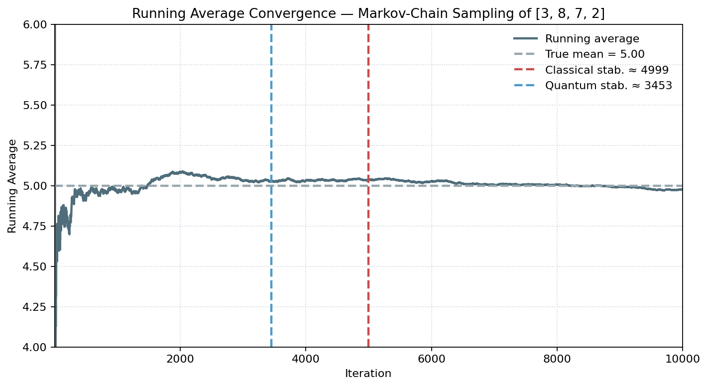
Simulation Example: Running Average Convergence

To illustrate the stabilization phenomenon, we simulate a 10,000-step run of the uniform “teleporting” Markov chain over the list [3, 8, 7, 2]. The plot shows the running average (solid line) converging toward the true mean (dashed line). Vertical dashed lines mark the expected stabilization times under the classical and quantum bounds.

Remarks and Stabilization Retention

Theorem 1 established a resource bound for achieving a stabilization window at a fixed horizon, essentially asking how many queries are needed so that $W$ consecutive estimates fall inside the target band with high probability. In many settings, however, one desires a stronger anytime guarantee: we do not fix the horizon in advance, but instead run the estimator until it naturally stabilizes, and then ask for assurances that once a window appears it truly reflects convergence.

The following theorem formulates this idea. By coupling an iterative amplitude-estimation schedule with a careful allocation of failure probability across rounds, we obtain stabilization that is valid uniformly over time. This reframes the problem: rather than bounding error at a single time, we bound the complexity of entering and retaining a valid window whenever it first occurs.

Theorem 2 (Windowed Quantum AE: Anytime Stabilization Guarantee)

Let $f:S\to[0,1]$ with mean $\mu=\mathbb{E}_\pi[f]$. An iterative amplitude estimation (AE) procedure produces sequential estimates $\hat\mu_{1},\hat\mu_{2},\ldots$. Define stabilization as $W$ consecutive outputs all lying in $[\mu-\delta,\mu+\delta]$.

There exists a schedule of AE calls such that, with probability at least $1-\beta$, the process eventually enters such a stabilization window and it persists for the full $W$ steps. The total query complexity is

$$\tilde{O}\!\left(\frac{1}{\delta}\,\log\frac{W}{\beta}\right).$$

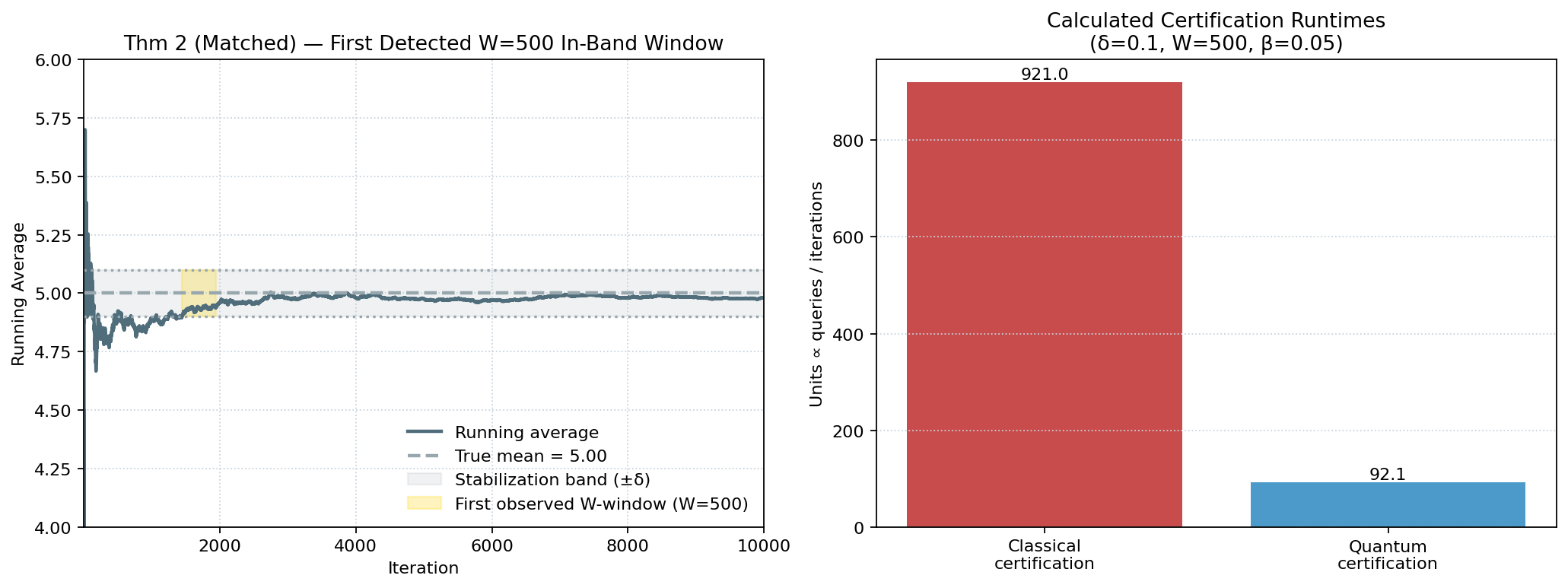
Simulation Example: Certified Stabilization (Theorem 2)

We run the same 10,000-step simulation of the uniform “teleporting” Markov chain over [3, 8, 7, 2] and visualize the certified stabilization guarantee. The left panel shows the running average (solid line) with a shaded stabilization band around the true mean (dashed line) using δ = 0.1. We then detect the first window of length W = 500 where the trajectory remains entirely within the band and highlight that window in maroon. This illustrates the Theorem 2 notion of persistence (staying in-band for W steps), which is stronger than the “first entry” view from Theorem 1.

The right panel compares the calculated certification runtimes to detect and certify such a window at confidence 1 − β (here β = 0.05): the classical detector scales like (1/δ²)·log(W/β), while the quantum WQAE detector scales like (1/δ)·log(W/β), showing the quadratic savings in 1/δ for the quantum procedure (same color scheme as elsewhere).