Unified manuscript
Distribution-Controlled Selective Quantization
Distortion, allocation, and margin-survival accuracy curves for a distribution-shaping view of mixed-precision quantization.
1. The Question
Quantization buys cheaper storage and arithmetic by replacing high-precision parameters with lower-precision approximations. The blunt analysis treats the resulting error as if it can hit every coordinate at once with equal consequence. That is safe, but it misses the geometry of a trained model: some directions move the output a great deal, while others barely register on the data distribution.
Selective quantization asks not simply "how large is the rounding error?" but "where does that error land?" The right object is anisotropic: low precision should be allocated heavily to directions with small sensitivity, lightly to directions with large sensitivity, and smoothly or abruptly depending on the objective used to choose the allocation.
\[ \text{quantization schedule} \longrightarrow \text{cumulative distortion} \longrightarrow \text{margin survival} \longrightarrow \text{accuracy curve}. \]
Start with a linear readout \(f_w(x)=w^\top x+b\). Quantization perturbs each coordinate only when a selector \(M_i\) is active:
The data distribution enters through a sensitivity score such as \(s_i=\mathbb E_{\mathcal D}|X_i|\). The basic selective family is
so low-sensitivity directions receive more of the quantization mass. This changes the question from "how large is the rounding error?" to "where does the rounding error land?"
Distribution
Sensitivity scores measure how strongly the model uses each coordinate on the data it actually sees.
Allocation
Quantization probabilities and bit widths determine where low precision is applied.
Distortion
The relevant first-order term is the aligned product \(q_i\varepsilon_i s_i\), not the error scale alone.
2. Distribution-Controlled Gates
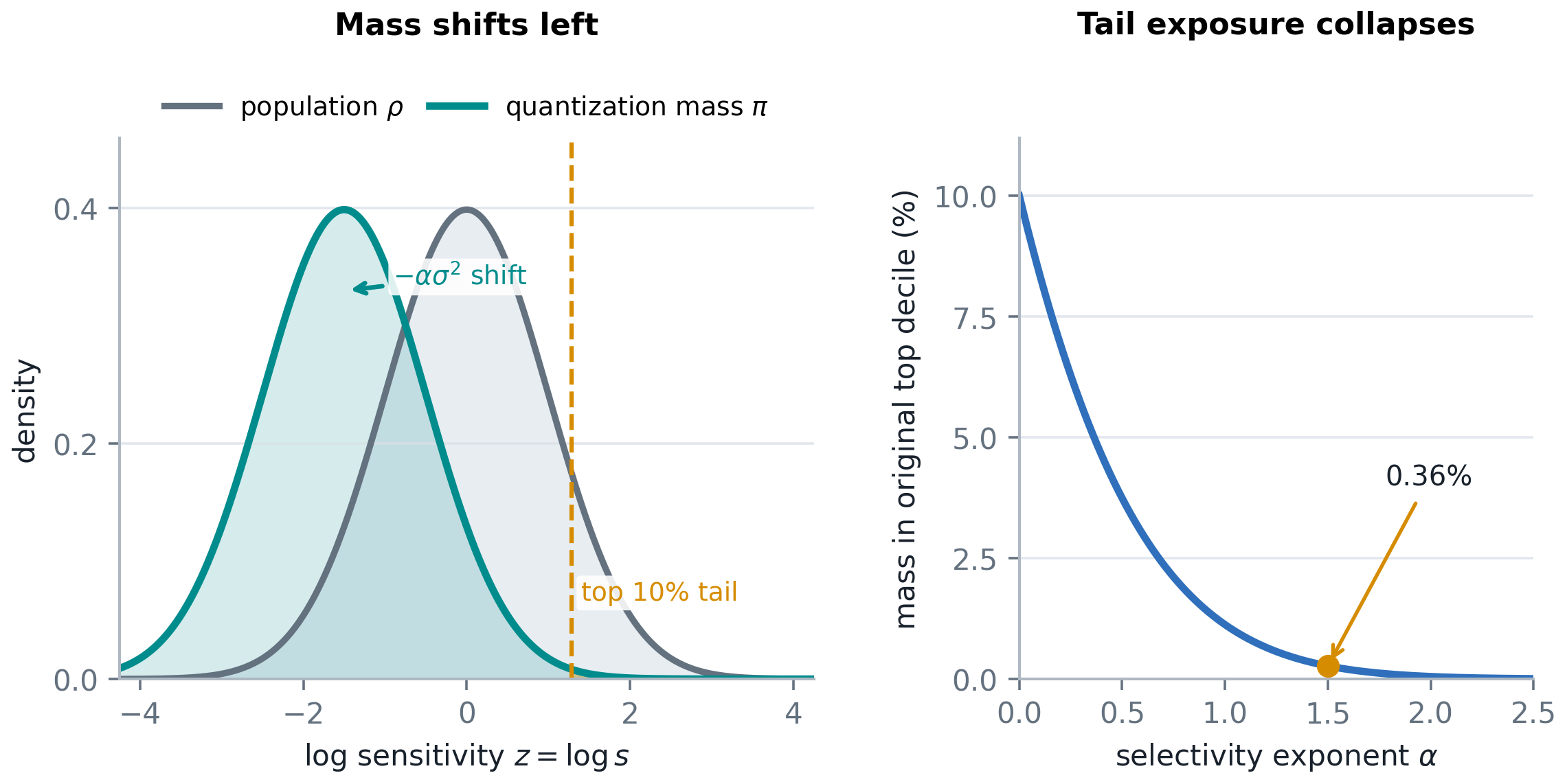
Let \(z=\log s\), and let \(\rho(z)\) be the population density of log-sensitivities. Applying a selective rule produces the quantization density
For a lognormal population and \(q(s)\propto s^{-\alpha}\), the quantization mass shifts left by \(\alpha\sigma^2\) in log-sensitivity. The high-sensitivity tail is still present in the model, but it receives very little of the low-precision budget.
3. First-Order Distortion
Proposition 1. Selective quantization bound
For every fixed input \(x\in\mathbb R^d\),
Averaging over \(X\sim\mathcal D\) gives
Uniform quantization sets \(q_i=q\) and \(\varepsilon_i=\varepsilon\), giving the coarser \(q\varepsilon\sum_i s_i+\varepsilon_b\). Selective quantization improves the same bound by moving mass to coordinates where the product is cheap.
Proposition 2. Budget-optimal selection
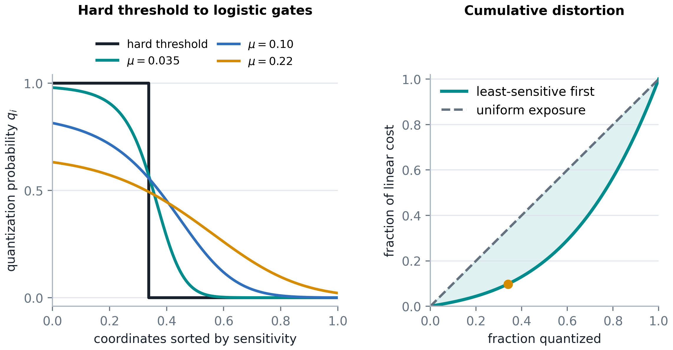
With common error scale \(\varepsilon_i=\varepsilon\) and budget \(\sum_iq_i=K\), minimizing \(\varepsilon\sum_i q_is_i\) places mass on the \(K\) least sensitive coordinates. If \(K\) is not an integer, one coordinate is fractional.
Smoothing the threshold
Abrupt rules are sometimes undesirable. They are hard to tune, brittle under noisy sensitivity estimates, and inconvenient when the selection mechanism is trained by gradient methods. Adding a convex entropy penalty softens the vertex solution:
Proposition 3. Smooth allocation
With \(c_i=\varepsilon_i s_i\) and \(\mu>0\), the unique minimizer is logistic in the coordinate cost:
where \(\nu\) is chosen so that \(\sum_i q_i^\star=K\). As \(\mu\to0\), the solution steepens into the threshold rule.
When signs matter
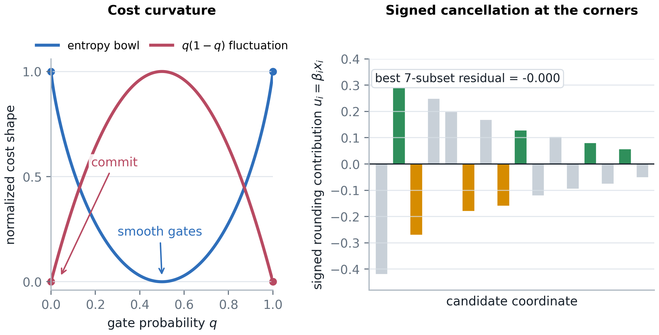
If quantization errors are independent, bounded, and mean zero, signed terms cancel and concentration gives a sharper tail. Deterministic rounding is different: the fixed signs make the bias term capable of cancellation, while the gate variance contains \(q_i(1-q_i)\), which is concave and vanishes at \(q_i=0\) and \(q_i=1\).
Proposition 4. Selection variance and tail
Let \(u_i=\beta_i x_i\) and \(Z(x)=\sum_iM_i u_i\), with \(M_i\sim\operatorname{Bernoulli}(q_i)\). Then
At deterministic vertices \(q_i\in\{0,1\}\), the gate variance disappears and the residual problem becomes choosing a subset whose signed rounding errors cancel.
The same argument lifts to ReLU networks by replacing coordinates with parameter blocks. If \(G_j\) is a local block sensitivity, then inside a visited activation region,
4. Distribution Shaping as Constrained Optimization
The allocation rule can be written as an explicit constrained problem. Given a target distortion \(\tau\), choose probabilities and bit widths to minimize memory:
A regularizer can shape the induced quantization distribution \(\pi_\phi(z)\), for example toward a uniform target, a lognormal target, or a mixture between them:
Proposition 5. Continuous-bit water filling
For distortion terms \(a_j2^{-b_j}\), memory weights \(m_jb_j\), and box constraints \(b_{\min}\le b_j\le b_{\max}\), the relaxed optimizer is
More sensitive or curvature-heavy blocks receive more bits; cheap blocks fall to the lower precision floor.
5. From Distortion to Margins
The preceding theory controls score movement. A classifier's accuracy is governed by whether that movement crosses decision margins. For a multiclass classifier with scores \(f_c(x)\), define the clean training margin of example \((x_i,y_i)\) by
The example is correctly classified when \(m_i>0\). After quantizing a cumulative set \(S_k\), write the score perturbation as \(\delta_c^{(k)}(x_i)=f_c^{(k)}(x_i)-f_c(x_i)\). The quantized margin obeys
For a linear score model, quantizing coefficient feature \(j\) changes class \(c\)'s score by \(\delta_c^{(k)}(x_i)=\sum_{j\in S_k}\Delta W_{cj}x_{ij}\). A schedule-level proxy replaces the sample-specific perturbation by cumulative first-order exposure:
Proposition 6. Accuracy as margin survival
Let \(S_k\) be a cumulative quantization schedule and let \(D(k)=\sum_{j\in S_k}c_j\). If the induced margin perturbation is approximated by a common scale factor times cumulative distortion, \(|\Delta m_i(k)|\approx\gamma D(k)\), then
where \(F_M\) is the empirical CDF of clean positive margins among initially correct training examples and \(A_0\) is full-precision training accuracy. With endpoint normalization to the fully quantized accuracy \(A_\infty=A(d)\),
\[ \text{accuracy curve} \approx \text{margin survival} \circ \text{cumulative quantization distortion}. \] The selective-quantization product supplies the distortion path \(D(k)\). The margin distribution turns that path into discrete classification errors.
6. Closed-Form Least-Sensitive-First Accuracy
Specialize to the least-sensitive-first schedule. Let \(\phi=k/d\) be the fraction of quantized coordinates and suppose coordinate costs are approximately lognormal:
The least-sensitive-first cumulative distortion fraction is
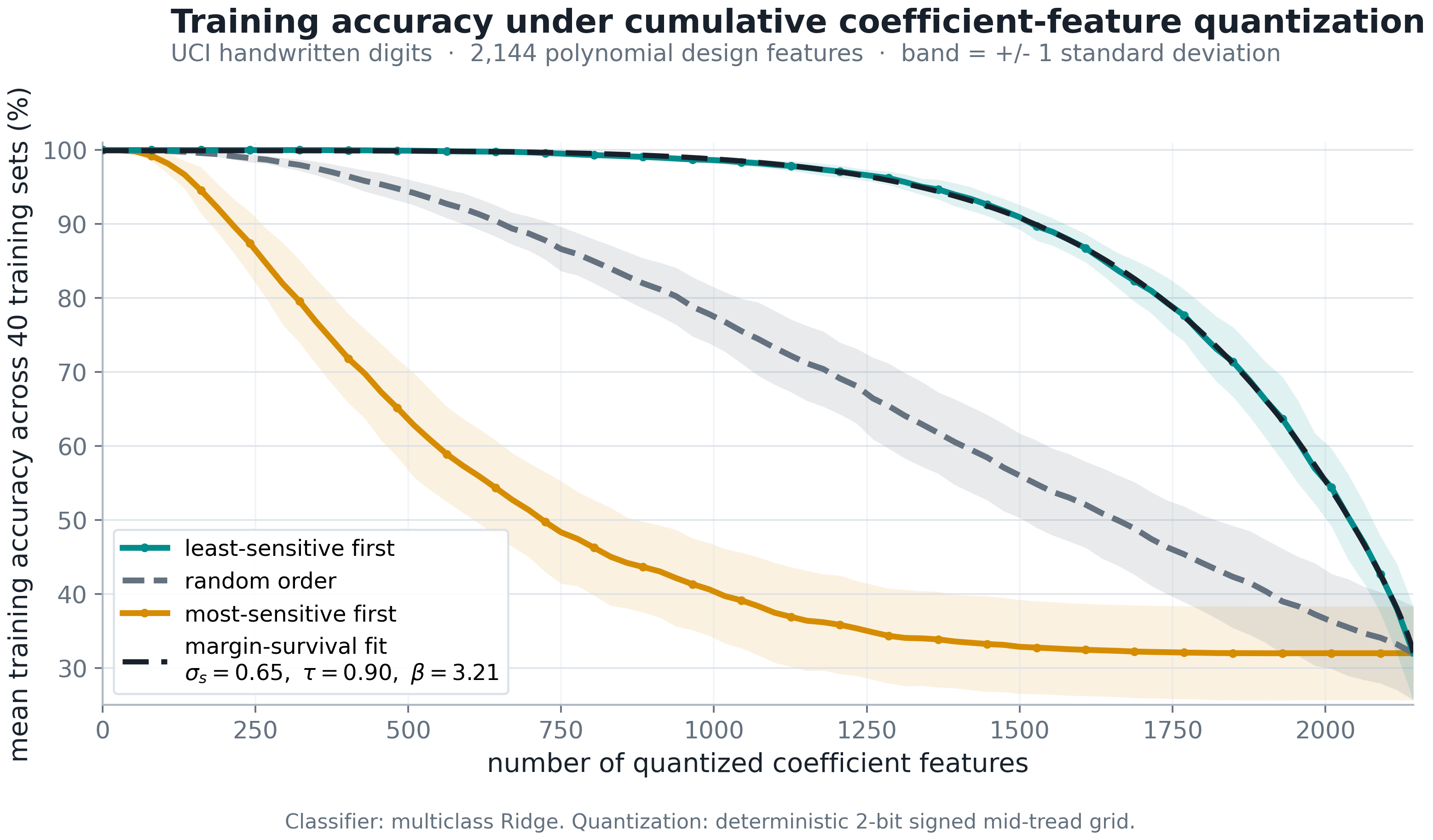
This is the plateau generator: a large fraction of coordinates can be quantized while accumulating only a small fraction of the total sensitivity-weighted distortion. Approximate the empirical margin CDF by a Weibull-type failure law,
Absorbing the margin scale into \(\tau\), composition gives the explicit least-sensitive-first accuracy curve
| Quantity | Symbol | Fitted value |
|---|---|---|
| Full-precision training accuracy | \(A_0\) | 99.923% |
| Fully quantized training accuracy | \(A_\infty\) | 32.065% |
| Log-cost spread | \(\sigma_s\) | 0.651 |
| Margin scale | \(\tau\) | 0.905 |
| Margin-shape exponent | \(\beta\) | 3.214 |
| Fit RMSE | - | 0.159 percentage points |
The fit is a structural check rather than a benchmark claim. The original formalism predicts that least-sensitive-first quantization accumulates distortion slowly. The margin formalism predicts that accuracy remains stable until cumulative distortion enters the body of the margin distribution. Together they explain the plateau-then-collapse shape.
Reproduction files: summary CSV, raw split CSV, and source figure PNG.

7. ReLU Net Experiment
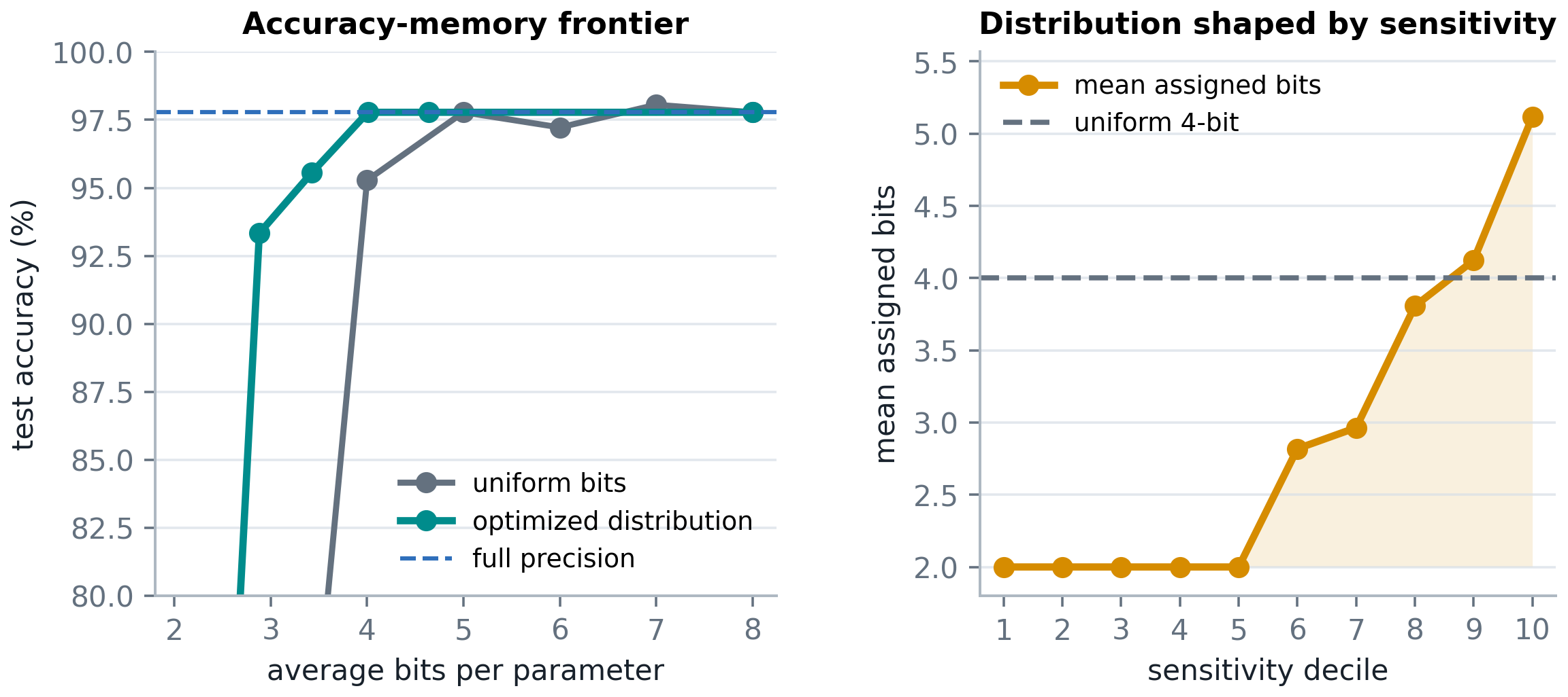
The paper includes a small post-training quantization test on the scikit-learn digits dataset. A ReLU classifier with architecture \(64\to 96\to 10\) is trained in full precision. Parameter sensitivity is estimated by
where \(\widehat F_i\) is an empirical diagonal Fisher estimate on a calibration split. The optimizer then chooses integer bits \(b_i\in\{2,\ldots,8\}\) subject to the same proxy distortion budget used by a uniform baseline.
| Policy | Average bits | Compression vs. fp32 | Test accuracy | Interpretation |
|---|---|---|---|---|
| Full precision | 32.00 | 1.00x | 97.8% | Reference model. |
| Uniform 4-bit | 4.00 | 8.00x | 95.3% | Same average memory as the strongest selective point, but lower accuracy. |
| Selective, target 6 | 4.01 | 7.98x | 97.8% | Matches full precision at roughly one eighth the fp32 memory. |
| Selective, target 5 | 3.43 | 9.34x | 95.6% | Beats uniform 4-bit accuracy with less memory. |
Reproduction files: results CSV, bit distribution bins, and experiment summary.
8. One Product, Five Geometries
\[ \sum_j q_j\,\varepsilon_j\,G_j \qquad \text{selection probability} \times \text{error scale} \times \text{sensitivity}. \] This product is the invariant. The allocation rule and the observed accuracy curve are determined by the curvature, constraints, and margin distribution built around it.
| Regime | Shape of objective or readout | Behavior |
|---|---|---|
| First-order magnitude | Linear in \(q_i\) | Vertex solution; quantize least-sensitive coordinates first. |
| Entropy-relaxed selection | Convex smoothing term | Interior logistic gates; threshold recovered as \(\mu\to0\). |
| Deterministic rounding | Concave fluctuation \(q_i(1-q_i)\) plus signed bias | Commit to corners, then choose subsets whose signed errors cancel. |
| Distribution control | Memory with loss constraint | Shape the quantization distribution along the Pareto frontier. |
| Margin survival | Thresholding by clean classification margins | Accuracy remains stable until cumulative distortion reaches the margin distribution. |
The practical message is stable across the variants: spend numerical imprecision where sensitivity is small. What changes is the mode of spending. Linear costs commit by a threshold, convex relaxations hedge smoothly, deterministic signed errors return the problem to combinatorial commitment, constrained optimization turns allocation into direct distribution control, and margins turn cumulative distortion into the observed accuracy curve.
References
- Y. LeCun, J. S. Denker, and S. A. Solla. Optimal Brain Damage. Advances in Neural Information Processing Systems, 1989.
- Z. Dong, Z. Yao, Y. Cai, D. Arfeen, A. Gholami, M. W. Mahoney, and K. Keutzer. HAWQ-V2: Hessian Aware trace-Weighted Quantization of Neural Networks. Advances in Neural Information Processing Systems, 2020.
- E. Frantar, S. Ashkboos, T. Hoefler, and D. Alistarh. GPTQ: Accurate Post-Training Quantization for Generative Pre-trained Transformers. International Conference on Learning Representations, 2023.
- S. Gupta, A. Agrawal, K. Gopalakrishnan, and P. Narayanan. Deep Learning with Limited Numerical Precision. International Conference on Machine Learning, 2015.
- C. Louizos, M. Welling, and D. P. Kingma. Learning Sparse Neural Networks through \(L_0\) Regularization. International Conference on Learning Representations, 2018.
- E. Jang, S. Gu, and B. Poole. Categorical Reparameterization with Gumbel-Softmax. International Conference on Learning Representations, 2017.
- T. M. Cover and J. A. Thomas. Elements of Information Theory. Wiley, 2nd edition, 2006.
- F. Pedregosa et al. Scikit-learn: Machine Learning in Python. Journal of Machine Learning Research, 2011.