Memoization does more than reduce work. It folds a recursion tree into a DAG, and the redundant work has a visible startup shape before it reaches its asymptotic speed. The paper's invariant is the velocity takeoff kernel: a compact way to see whether redundancy appears immediately, after a delay, through ringing, or along a slow diffusive tail. This exposes finite-response structure that standard first-order complexity summaries usually collapse into the same asymptotic growth rate.
Terminal speedusual asymptotic overlap velocity
Takeoff kernelfinite onset of redundant work
Separationsame limit, different startup physics
1. What Memoization Exposes
Start with a recursive computation on input size \(n\). Let \(N_n\) count calls in the naive recursion tree, where repeated subproblems are counted each time they appear. Let \(M_n\) count the distinct subproblem labels left after memoization identifies repeats. The overlap ratio \(\Theta_n\), logarithmic overlap \(S_n\), and overlap velocity \(v_n\) are
The overlap velocity \(v_n\) tracks how quickly memoizable redundancy is being created as \(n\) grows. It splits cleanly into tree velocity minus DAG velocity:
If \(\log N_n \sim \alpha n\) and \(\log M_n \sim \beta n\), where \(\alpha\) is the tree growth exponent and \(\beta\) is the memoized-DAG growth exponent, then \(v_n \to \alpha-\beta\). That limiting number is useful, but it misses the finite story: how does redundancy actually turn on?
startup: little visible overlaptoterminal overlap speed \(\alpha-\beta\)
2. The Finite-Lag Model
A finite-lag recursive schema has a finite set of positive decrements \(J\), with \(a_j\) calls from size \(n\) to size \(n-j\) for each \(j\in J\). This gives a clean laboratory for studying takeoff: the naive tree size follows
\[
N_n = 1+\sum_{j\in J} a_j N_{n-j},
\qquad n \ge 1,
\qquad N_m=1 \text{ for } m\le 0 .
\]
The total branching number is \(A=\sum_{j\in J}a_j\). In the redundant case \(A\gt1\), define the characteristic polynomial \(Q\) in the variable \(z\), its positive root \(\rho\), and the terminal tree speed \(\alpha\) by
The root \(\rho\in(0,1)\) sets the terminal tree speed \(\alpha\). The raw recursion kernel \(K_j=a_j/A\) says where branches land; the takeoff kernel asks a different question: how the observed velocity approaches \(\alpha\).
3. The Takeoff Kernel
Normalize the tree velocity by its terminal value. The result is a finite-response profile \(F_n\), and the kernel \(\kappa\) is the causal finite difference that drives it.
Equivalently, the profile is the step response of the kernel. Here \(H^{\mathrm{step}}\) is the discrete step function, equal to \(1\) for nonnegative indices and \(0\) for negative indices:
For an aperiodic finite-lag recurrence, \(u_n\to\alpha\). The kernel has total mass one, and for some constants \(C\gt0\) and \(0\lt\lambda\lt1\), its tail decays exponentially:
The modes come from non-dominant singularities \(\zeta\) of the tree-size generating function, including non-dominant roots of \(Q\) and affine boundary contributions such as \(z=1\). Correction terms scale like \((\rho/\zeta)^n\). Positive real modes give smoothing; negative or complex modes give alternating or oscillatory takeoff.
The modal radius \(\lambda_\star\) records the slowest visible transient among those non-dominant singularities \(\zeta\):
When \(\lambda_\star\) is small, velocity settles fast. When \(\lambda_\star\) is near one, the recursion can spend a long finite window behaving unlike its asymptotic limit.
4. Same Limit, Different Takeoff
The main theorem says the kernel is not merely decorative. Two schemas can share terminal tree speed, polynomial memoized state growth, and limiting overlap velocity, yet still take off in sharply different ways.
Main separation
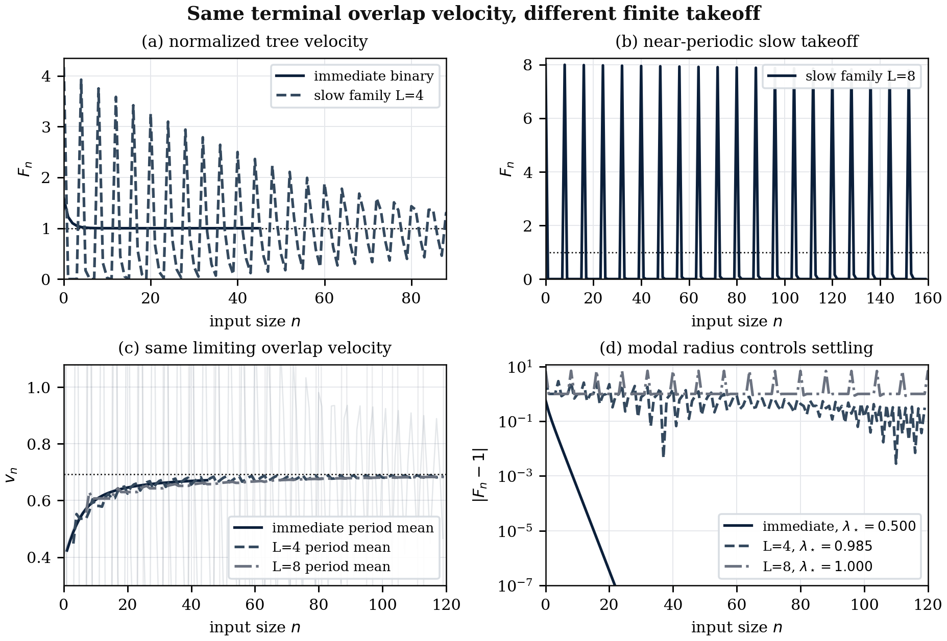
There are finite-lag schemas with \(\alpha=\log 2\), \(M_n=O(n)\), and limiting overlap velocity \(\log 2\), but with different takeoff classes. Here \(O(n)\) means at most linear growth up to constants, and \(\delta\gt0\) is an arbitrary tolerance. Immediate binary recursion settles fast; a delayed aperiodic family can have modal radius greater than \(1-\delta\).
The dominant root is still \(\rho=1/2\), so the terminal speed remains \(\log2\). But as \(L\) grows, a non-dominant root \(\zeta_L\) moves close to the dominant circle, forcing the modal radius toward one.
Separation in one picture. The terminal overlap velocity is the same, but the finite response is not: immediate takeoff versus long near-periodic ringing.
5. Terminal Speed as Entropy per Decrement
The terminal speed also has a compact information-theoretic form. For a probability distribution \(p=(p_j)_{j\in J}\) over decrements \(J\), define entropy \(H(p)\), mismatch from the branch kernel \(K\), and mean decrement \(\mu(p)\):
Read this as branching entropy per unit input size after paying a mismatch penalty. The takeoff kernel adds what this terminal formula cannot: the route by which the terminal speed becomes visible.
6. Takeoff Types
The kernel gives a vocabulary for recursive redundancy. These are the practical signatures to look for in traces.
No takeoff
One recursive call, \(A=1\). The tree is path-like: there is stack depth, but no positive exponential overlap velocity.
Immediate takeoff
Binary one-step recursion has \(\alpha=\log2\). Redundancy appears almost immediately, up to boundary effects.
Delayed takeoff
Binary lag \(L\) has \(\alpha=(\log2)/L\). In the original coordinate, recursive mass must pay the lag before it returns.
Leading ringing
Near-periodic delayed branching creates complex modes close to the dominant circle, producing long damped oscillations.
Mixed-stage smoothing
Parallel fast and slow channels do not simply add. Their roots interact, producing a fast rise followed by a slower settling tail.
Diffusive smoothing
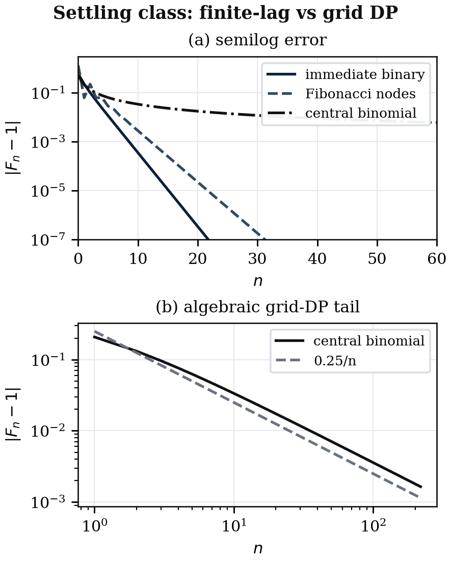
Grid dynamic programs can have algebraic \(1/n\)-scale tails instead of exponential finite-lag settling.
Fibonacci is a boundary-convention lesson
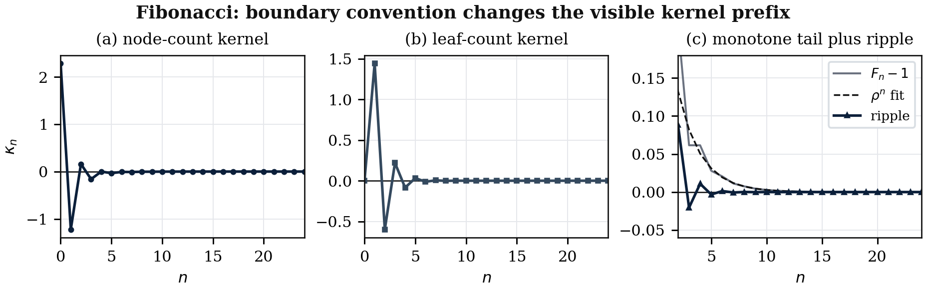
Naive Fibonacci has \(J=\{1,2\}\), \(a_1=a_2=1\), and terminal speed \(\alpha=\log\varphi\), where \(\varphi=(1+\sqrt5)/2\) is the golden ratio. Under node counting, the affine \(+1\) contributes a monotone \(z=1\) correction; under leaf counting, the alternating mode moves into clearer view.
Fibonacci takeoff. The tail modes come from the same recurrence, but the visible kernel prefix changes when the counting convention changes.
Finite-lag versus grid-DP tails
For diagonal lattice paths, let \(P_{n,n}\) be the number of paths to the grid point \((n,n)\). Then \(P_{n,n}=\binom{2n}{n}\), so velocity approaches its limit with algebraic correction rather than exponential correction:
If \(u_n\) has terminal value \(\alpha\), form \(F_n=u_n/\alpha\) and \(\kappa_n=F_n-F_{n-1}\). Plotting the kernel reveals the response class: immediate, delayed, oscillatory, mixed, or diffusive.
When the DAG velocity \(w_n\) also has a positive terminal value \(\beta\), define its normalized profile by \(G_n=w_n/\beta\). Then the overlap velocity decomposes as
When \(M_n\) is polynomial, \(\beta=0\), so overlap takeoff inherits tree takeoff. When the DAG itself grows exponentially, observed overlap becomes a difference between two response curves.
Practical read
For tolerance \(\varepsilon\gt0\), let \(T_\varepsilon\) be the first index after which \(|F_n-1|\le\varepsilon\) remains true. If the input range lies below \(T_\varepsilon\), asymptotic overlap exists but is not yet what the computation sees. If the range extends well beyond \(T_\varepsilon\), memoization is exposing persistent redundancy rather than boundary effects alone.
Conclusion
The limiting overlap velocity \(\alpha-\beta\) is the terminal reading of a richer finite-response object. The takeoff kernel records when memoizable redundancy becomes visible, how it settles, and whether it smooths, delays, rings, mixes stages, or diffuses.
The main separation is the point: first-order overlap invariants do not determine takeoff. The exponential tree growth, memoized state count, and limiting overlap velocity can all agree, while the startup response remains distinct.
That makes recursive redundancy feel less like a single cost number and more like a response curve. Once the curve is visible, memoization is not just a trick for saving calls; it becomes a lens on the hidden shape of repeated computation.